Left ventricular hypertrophy segmentation

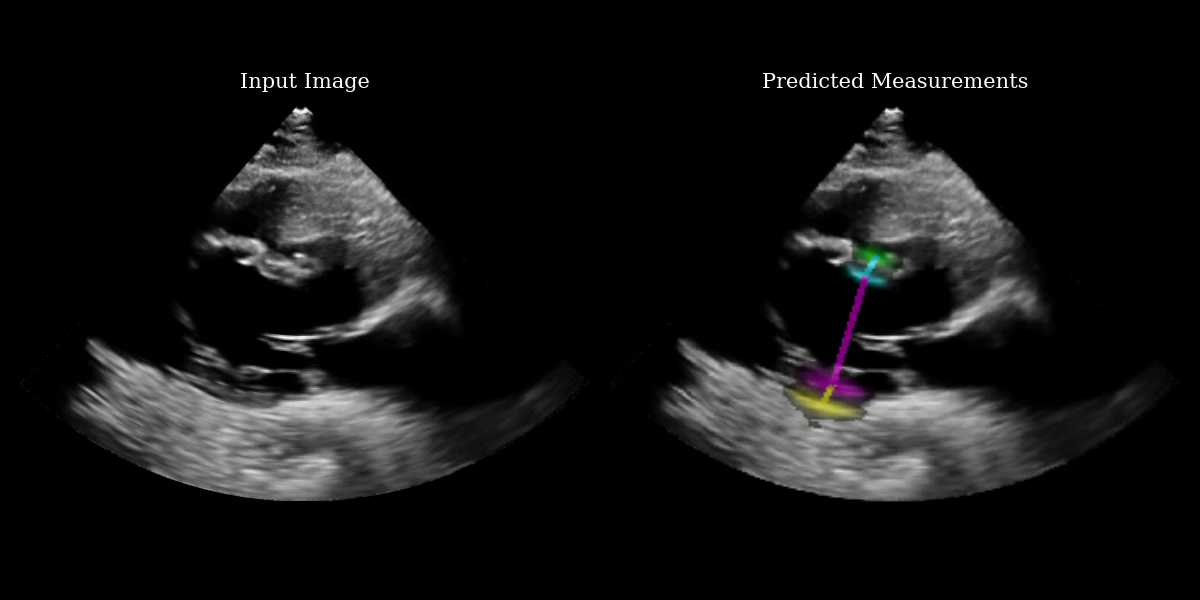
In this example we use the EchoNetLVH model to identify key points for measuring left ventricular hypertrophy from parasternal long axis echocardiograms. For more information on the method, see the original paper:

• Duffy, G., Cheng, P. P., Yuan, N., He, B., Kwan, A. C., Shun-Shin, M. J., … & Ouyang, D. (2022). High-throughput precision phenotyping of left ventricular hypertrophy with cardiovascular deep learning. JAMA cardiology, 7(4), 386-395.

   

‼️ Important: This notebook is optimized for GPU/TPU. Code execution on a CPU may be very slow.

If you are running in Colab, please enable a hardware accelerator via:

Runtime → Change runtime type → Hardware accelerator → GPU/TPU 🚀.

%%capture
%pip install zea

import os

os.environ["KERAS_BACKEND"] = "jax"
os.environ["TF_CPP_MIN_LOG_LEVEL"] = "3"

import matplotlib.pyplot as plt
from keras import ops
from PIL import Image
import numpy as np
import requests
from io import BytesIO

from zea import init_device
from zea.visualize import set_mpl_style

init_device(verbose=False)
set_mpl_style()

zea: Using backend 'jax'

# NOTE: this is a synthetic PLAX view image generated by a diffusion model.
url = "https://raw.githubusercontent.com/tue-bmd/zea/main/docs/source/notebooks/assets/plax.png"
response = requests.get(url)
img = Image.open(BytesIO(response.content)).convert("RGBA")

# Split channels
r, g, b, a = img.split()

# Composite onto a black background (RGB = 0,0,0)
black_bg = Image.new("RGBA", img.size, (0, 0, 0, 255))
img = Image.alpha_composite(black_bg, img)

# Convert to grayscale
img = img.convert("L")

# Convert to numpy
img_np = np.asarray(img).astype(np.float32)

from zea.models.echonetlvh import EchoNetLVH

# Load model from zeahub
model = EchoNetLVH.from_preset("echonetlvh")

# Add batch + channel dims
batch = ops.convert_to_tensor(img_np[None, ..., None])

# apply model to image, producing logits
logits = model(batch)

# use visualization function to visualize heatmaps and measurement lines on the input image
images_with_measurements = model.visualize_logits(batch, logits)

# Plotting
fig, (ax1, ax2) = plt.subplots(1, 2, figsize=(12, 6))

# Plot input image
ax1.imshow(img_np, cmap="gray")
ax1.set_title("Input Image", fontsize=15)
ax1.axis("off")

# Plot output with measurements
ax2.imshow(images_with_measurements[0])
ax2.set_title("Predicted Measurements", fontsize=15)
ax2.axis("off")

plt.tight_layout()
plt.savefig("echonetlvh_output.png")
plt.close()

Extracting the measurement points

The EchoNetLVH model ouptuts 4 heatmaps – one for each key point. The heatmaps indicate the probability that each pixel contains the key point. Because of this, we need a function to extract the key point from a given heatmap. There are various ways to do this – we implement a center-of-mass approach, preserving differentiability.

What we print below is the set of key points represented as indices with respect to the input image matrix.

key_points = ops.cast(model.extract_key_points_as_indices(logits)[0], "int")
measurement_keys = ["LVPW", "LVID", "IVS"]
print("Measurement type: [H1, W1] -> [H2, W2]")
for i in range(3):
    print(f"{measurement_keys[i]}: {key_points[i]} -> {key_points[i + 1]}")

Measurement type: [H1, W1] -> [H2, W2]
LVPW: [299 217] -> [287 226]
LVID: [287 226] -> [182 286]
IVS: [182 286] -> [187 281]