Task-based transmit beamforming perception-action loop
In this example we will implement a task-based perception-action loop that drives the transmit beamforming pattern towards gaining information about a downstream task variable of interest. We use the left-ventricular inner dimension (LVID), as measured by EchoNetLVH, as our downstream task variable.
![]()
‼️ Important: This notebook is optimized for GPU/TPU. Code execution on a CPU may be very slow.
If you are running in Colab, please enable a hardware accelerator via:
Runtime → Change runtime type → Hardware accelerator → GPU/TPU 🚀.
This notebook steps through a single iteration of the perception-action loop, going from a sparse acquisition \(\rightarrow\) a belief distribution over LVID values \(\rightarrow\) the transmit pattern for the next sparse acquisition. The steps for this loop are illustrated in the following diagram:
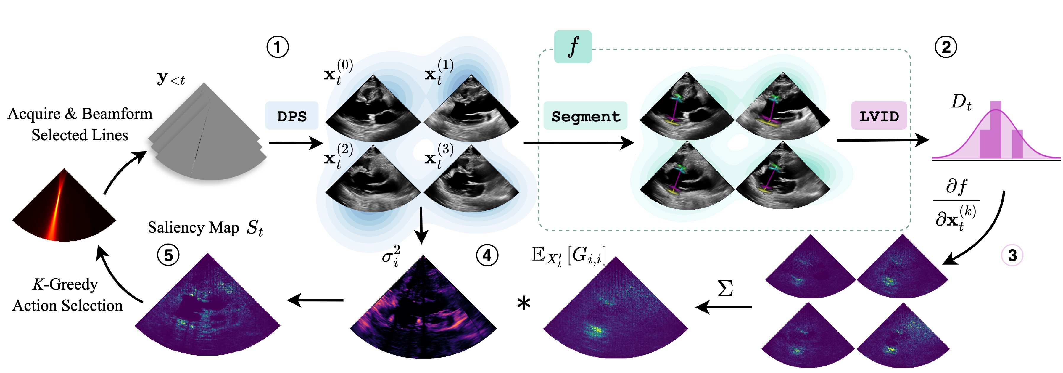
Generate a set of posterior samples from the sparse acquisition using Diffusion Posterior Sampling (DPS).
Pass each posterior sample \(x^{(i)}_t\) through the downstream task model \(f\) to produce samples from the downstream task distribution.
Compute the Jacobian matrix using each of the posterior samples as inputs.
Average those Jacobian matrices and multiply them with the pixel-wise variance of the input images to produce the downstream task saliency map.
Apply K-Greedy Minimization to select \(K\) scan lines for the next acquisition.
[1]:
%%capture
%pip install zea
Setup / Imports
[2]:
import os

os.environ["KERAS_BACKEND"] = "jax"
os.environ["TF_CPP_MIN_LOG_LEVEL"] = "3"

import matplotlib.pyplot as plt
from keras import ops
from PIL import Image
import numpy as np
import requests
from io import BytesIO

from zea import init_device
from zea.visualize import set_mpl_style
from zea.display import scan_convert_2d, inverse_scan_convert_2d
from zea.func import translate
from zea.visualize import plot_image_grid
from zea.io_lib import matplotlib_figure_to_numpy, save_video

init_device(verbose=False)
set_mpl_style()
zea: Using backend 'jax'
[3]:
n_prior_steps = 500
n_posterior_steps = 500
n_particles = 4
Load the target data
[4]:
# NOTE: this is a synthetic PLAX view image generated by a diffusion model.
url = "https://raw.githubusercontent.com/tue-bmd/zea/main/docs/source/notebooks/assets/plax.png"
response = requests.get(url)
img = Image.open(BytesIO(response.content)).convert("RGBA")
# Split channels
r, g, b, a = img.split()
# Composite onto a black background (RGB = 0,0,0)
black_bg = Image.new("RGBA", img.size, (0, 0, 0, 255))
img = Image.alpha_composite(black_bg, img)
img = img.convert("L")
img_np = np.asarray(img).astype(np.float32)
img_tensor = ops.convert_to_tensor(img_np)
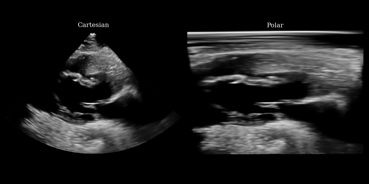
img_polar = inverse_scan_convert_2d(img_tensor, image_range=(0, 255))
img_polar_np = ops.convert_to_numpy(img_polar)
# plotting
fig, (ax1, ax2) = plt.subplots(1, 2, figsize=(12, 6))
ax1.imshow(img_np, cmap="gray")
ax1.set_title("Cartesian", fontsize=15)
ax1.axis("off")
ax2.imshow(img_polar_np, cmap="gray")
ax2.set_title("Polar", fontsize=15)
ax2.axis("off")
plt.tight_layout()
plt.savefig("cartesian_polar.png")
plt.close()
Define the downstream task function
[5]:
from zea.models.echonetlvh import EchoNetLVH

# First, load the downstream task model (EchoNetLVH in this case) from zeahub
echonetlvh_model = EchoNetLVH.from_preset("echonetlvh")
[6]:
# We need to precompute the scan conversion coordinates so that the
# scan conversion function is differentiable
from zea.display import compute_scan_convert_2d_coordinates

# set some parameters for scan conversion
n_rho = 224
n_theta = 224
rho_range = (0, n_rho)
theta_range = (np.deg2rad(-45), np.deg2rad(45))
resolution = 1.0
fill_value = 0.0
image_shape = (n_rho, n_theta)
pre_computed_coords, _ = compute_scan_convert_2d_coordinates(
    image_shape,
    rho_range,
    theta_range,
    resolution,
)


def lvid_downstream_task(posterior_sample):
    """
    Computes the LVID measurement from a posterior sample generated by the diffusion model.

    Params:
        posterior_sample (tensor of shape [H, W]) - should be a single posterior
            sample, not a batch, to preserve scalar output for differentiability
            using backprop.

    Returns:
        lvid_length (float)

    NOTE: we leverage that our downstream task variable is a scalar here to use simple autograd
    to compute our jacobian values. For multivariate downstream task variables, you'll need
    to compute the full jacobian, or approximate it, using functions like `jax.jvp`.
    """
    assert len(ops.shape(posterior_sample)) == 2  # Should just be [H, W]
    # First we need to pre-process the posterior sample from the diffusion model
    # so that it becomes a valid input to EchoNetLVH.
    posterior_sample_normalized = translate(ops.clip(posterior_sample, -1, 1), (-1, 1), (0, 255))
    posterior_sample_sc, _ = scan_convert_2d(
        posterior_sample_normalized, coordinates=pre_computed_coords, fill_value=fill_value
    )
    posterior_sample_sc_resized = ops.image.resize(
        posterior_sample_sc[None, ..., None], (224, 224)
    )  # model expects batch and channel dims
    logits = echonetlvh_model(posterior_sample_sc_resized)
    key_points = echonetlvh_model.extract_key_points_as_indices(logits)[0]
    lvid_bottom_coords, lvid_top_coords = key_points[1], key_points[2]
    lvid_length = ops.squeeze(ops.sqrt(ops.sum((lvid_top_coords - lvid_bottom_coords) ** 2)))
    return lvid_length


def animate_samples(samples, filename, title, fps=3):
    samples = translate(ops.clip(samples, -1, 1), (-1, 1), (0, 255))
    # bring frame dim to front
    samples = ops.moveaxis(samples, -1, 0)

    frames = []
    for i in range(len(samples)):
        fig, _ = plot_image_grid(
            samples[i],
            suptitle=title,
            vmin=0,
            vmax=255,
            cmap="gray",
        )
        frames.append(matplotlib_figure_to_numpy(fig))
        plt.close()
    save_video(frames, filename, fps=fps)
Simulate a sparse acquisition
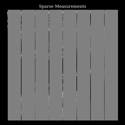
We simulate acquiring a sparse set of focused transmits and beamforming to single columns of lines by simply masking the target image to reveal only certain lines of pixels.
[7]:
from zea.agent.selection import EquispacedLines

fully_sampled_image = ops.image.resize(
    ops.convert_to_tensor(img_polar_np[None, ..., None]), (256, 256)
)
fully_sampled_image_normalized = translate(
    fully_sampled_image, range_from=(0, 255), range_to=(-1, 1)
)

img_shape = (256, 256)
line_thickness = 1
factor = 32
equispaced_sampler = EquispacedLines(
    n_actions=img_shape[1] // line_thickness // factor,
    n_possible_actions=img_shape[1] // line_thickness,
    img_width=img_shape[1],
    img_height=img_shape[0],
)

_, mask = equispaced_sampler.sample()
mask = ops.expand_dims(mask, axis=-1)

measurements = ops.where(mask, fully_sampled_image_normalized, 0.0)
[8]:
fig, ax = plt.subplots(figsize=(5, 5))
im = ax.imshow(measurements[0, ..., 0], cmap="gray", vmin=-1, vmax=1)
ax.set_title("Sparse Measurements")
ax.axis("off")
plt.tight_layout()
plt.savefig("measurements.png")
plt.close(fig)
Perception step
First we place the measurements and mask in a 3-frame buffer, since our EchoNetLVH diffusion model is a 3-frame model.
[9]:
measurement_buffer = ops.concatenate((ops.zeros((1, *img_shape, 2)), measurements), axis=-1)
mask_buffer = ops.concatenate((ops.zeros((1, *img_shape, 2)), mask), axis=-1)
Next, we load (automatically downloaded from the Hugging Face Hub) the diffusion model. We can first quickly sample from the prior \(\mathbf{x} \sim p(\mathbf{x})\) to see what kinds of images the model has learned to generate.
[10]:
from zea.models.diffusion import DiffusionModel

diffusion_model = DiffusionModel.from_preset("diffusion-echonetlvh-3-frame")

prior_samples = diffusion_model.sample(
    n_samples=n_particles,
    n_steps=n_prior_steps,
)
animate_samples(
    prior_samples,
    "./task_based_prior_samples.gif",
    title=r"Prior samples $x\sim p(x)$",
    fps=9,
)
500/500 ━━━━━━━━━━━━━━━━━━━━ 30s 44ms/step
zea: Successfully saved GIF to -> task_based_prior_samples.gif
That looks correct, we now proceed with posterior sampling to generate some samples from the Bayesian posterior \(\{\mathbf{x}_t^{(i)}\}_{i=0}^{N_p} \sim p(X_t \mid \mathbf{y}_{<t})\).
[11]:
posterior_samples = diffusion_model.posterior_sample(
    measurements=measurement_buffer,
    mask=mask_buffer,
    n_samples=n_particles,
    n_steps=n_posterior_steps,
    initial_step=0,
    omega=10,
)
animate_samples(
    posterior_samples[0],  # posterior samples has an extra batch dim of length measurements
    "./task_based_posterior_samples.gif",
    title=r"Posterior samples $x\sim p(x | y)$",
    fps=9,
)
zea: Successfully saved GIF to -> task_based_posterior_samples.gif
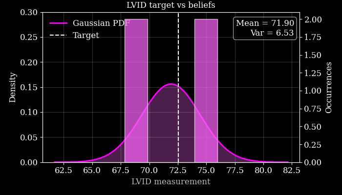
Next we use these posterior samples to derive downstream task posterior samples, i.e. beliefs about the value of the LVID. We then compare this to the target LVID measured from the ground-truth in order to see how accurate the agent’s beliefs are.
We also plot this visually, quantifying our downstream uncertainty using Gaussian variance.
[12]:
# First let's measure the ground truth LVID from the fully-sampled target image
target_lvid = lvid_downstream_task(fully_sampled_image_normalized[0, ..., 0])

# Then we can pass each posterior sample through the lvid measurement function
lvid_posterior = ops.vectorized_map(
    lambda ps: ops.vectorized_map(lambda p: lvid_downstream_task(p[..., -1]), ps), posterior_samples
)

print(f"Target LVID: {target_lvid}")
print(f"Agent's LVID beliefs: {lvid_posterior}")
Target LVID: 72.5322036743164
Agent's LVID beliefs: [[69.403465 68.92208  75.11672  74.17236 ]]
[13]:
import numpy as np
import matplotlib.pyplot as plt
from scipy.stats import norm

samples = ops.convert_to_numpy(lvid_posterior).flatten()

# --- fit Gaussian ---
mu = np.mean(samples)
sigma = np.std(samples, ddof=1)

# make it a bit taller/thinner if desired
sigma *= 0.8

# --- x grid for PDF ---
x = np.linspace(mu - 4 * sigma, mu + 4 * sigma, 400)
pdf = norm.pdf(x, mu, sigma)

fig, ax_density = plt.subplots(figsize=(7, 4))

# ---- Density axis (left) ----
ax_density.set_ylabel("Density", color="white")
ax_density.set_ylim(0, 0.3)
ax_density.plot(x, pdf, color="#FF00FF", lw=2, label="Gaussian PDF")
ax_density.fill_between(x, pdf, color="#FF66FF", alpha=0.3)

# Target line
ax_density.axvline(target_lvid, color="white", linestyle="--", lw=1.5, label="Target")

# ---- Occurrences axis (right) ----
ax_counts = ax_density.twinx()
ax_counts.set_ylabel("Occurrences", color="white")
ax_counts.set_ylim(0, 2.1)  # manually cap at 2 occurrences
ax_counts.hist(
    samples,
    bins=10,
    range=(x.min(), x.max()),
    color="#FF66FF",
    edgecolor="white",
    alpha=0.7,
    zorder=2,
)

# Mean/variance text
ax_density.text(
    0.98,
    0.95,
    f"Mean = {mu:.2f}\nVar = {sigma**2:.2f}",
    ha="right",
    va="top",
    transform=ax_density.transAxes,
    fontsize=12,
    color="white",
    bbox=dict(boxstyle="round,pad=0.3", fc="black", ec="white", alpha=0.6),
)

ax_density.set_xlabel("LVID measurement")
ax_density.legend(frameon=False, loc="upper left")
ax_density.grid(alpha=0.2, color="white")
plt.tight_layout()
plt.title("LVID target vs beliefs")
plt.savefig("lvid_target_beliefs.png")
plt.close()
Action step
Finally, we can use our posterior samples and downstream task function to identify the regions of the image space that should be measured in the next sparse acquisition, in order to gain information about the LVID. For this we can use the TaskBasedLines function from zea.agent.selection, as follows:
[14]:
from zea.agent.selection import TaskBasedLines

agent = TaskBasedLines(
    n_actions=img_shape[1] // line_thickness // factor,
    n_possible_actions=img_shape[1] // line_thickness,
    img_width=img_shape[1],
    img_height=img_shape[0],
    downstream_task_function=lvid_downstream_task,
)
selected_lines_k_hot, mask, pixelwise_contribution_to_var_dst = agent.sample(
    posterior_samples[..., -1]
)
[15]:
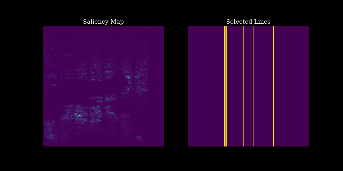
# plotting
fig, (ax1, ax2) = plt.subplots(1, 2, figsize=(12, 6))

# Plot output with measurements
ax1.imshow(pixelwise_contribution_to_var_dst[0] ** 0.5)  # rescale by sqrt for visualization
ax1.set_title("Saliency Map", fontsize=15)
ax1.axis("off")

# Plot input image
ax2.imshow(mask[0])
ax2.set_title("Selected Lines", fontsize=15)
ax2.axis("off")

plt.savefig("task_based_selection.png")
plt.close()