Simulating ultrasound data with zea

This notebook demonstrates how to simulate ultrasound RF data using the zea toolbox. We’ll define a probe, a scan, and a simple phantom, then use the simulator to generate synthetic RF data. Finally, we’ll visualize the results and show how to process the simulated data with a zea pipeline.

 

‼️ Important: This notebook is optimized for GPU/TPU. Code execution on a CPU may be very slow.

If you are running in Colab, please enable a hardware accelerator via:

Runtime → Change runtime type → Hardware accelerator → GPU/TPU 🚀.

%%capture
%pip install zea

import os

os.environ["KERAS_BACKEND"] = "jax"
os.environ["ZEA_DISABLE_CACHE"] = "1"

import matplotlib.pyplot as plt
import numpy as np

import zea
from zea import init_device
from zea.simulator import simulate_rf
from zea.probes import Probe
from zea.scan import Scan
from zea.beamform.delays import compute_t0_delays_planewave
from zea.visualize import set_mpl_style
from zea.beamform import phantoms

zea: Using backend 'jax'

init_device(verbose=False)
set_mpl_style()

Let’s define a helper function to plot RF data.

def plot_rf(rf_data, title="RF Data", cmap="gray"):
    """Plot the first transmit and first channel of the RF data."""
    plt.figure(figsize=(8, 4))
    plt.imshow(
        rf_data[0, :, :, 0].T,
        aspect="auto",
        cmap=cmap,
        extent=[0, rf_data.shape[1], 0, rf_data.shape[2]],
    )
    plt.xlabel("Sample (axial)")
    plt.ylabel("Element (lateral)")
    plt.title(title)
    plt.colorbar(label="Amplitude")
    plt.tight_layout()
    plt.savefig("simulation_plot_rf.png")
    plt.close()

Define zea.Probe and zea.Scan

We’ll use a linear probe and a simple planewave scan for this simulation. Let’s start with the probe definition.

# Define a linear probe
n_el = 64
aperture = 20e-3
probe_geometry = np.stack(
    [np.linspace(-aperture / 2, aperture / 2, n_el), np.zeros(n_el), np.zeros(n_el)], axis=1
)

probe = Probe(
    probe_geometry=probe_geometry,
    center_frequency=5e6,
    sampling_frequency=20e6,
)

Now we’ll define the necessary parameters for the scan object.

# Define a planewave scan
n_tx = 3
angles = np.linspace(-5, 5, n_tx) * np.pi / 180
sound_speed = 1540.0

# Set grid and image size
xlims = (-20e-3, 20e-3)
zlims = (10e-3, 35e-3)
width, height = xlims[1] - xlims[0], zlims[1] - zlims[0]
wavelength = sound_speed / probe.center_frequency
grid_size_x = int(width / (0.5 * wavelength)) + 1
grid_size_z = int(height / (0.5 * wavelength)) + 1

t0_delays = compute_t0_delays_planewave(
    probe_geometry=probe_geometry,
    polar_angles=angles,
    sound_speed=sound_speed,
)
tx_apodizations = np.ones((n_tx, n_el)) * np.hanning(n_el)[None]

Now we can initialize the scan object with the defined parameters.

scan = Scan(
    n_tx=n_tx,
    n_el=n_el,
    center_frequency=probe.center_frequency,
    sampling_frequency=probe.sampling_frequency,
    probe_geometry=probe_geometry,
    t0_delays=t0_delays,
    tx_apodizations=tx_apodizations,
    element_width=np.linalg.norm(probe_geometry[1] - probe_geometry[0]),
    focus_distances=np.ones(n_tx) * np.inf,
    polar_angles=angles,
    initial_times=np.ones(n_tx) * 1e-6,
    n_ax=1024,
    xlims=xlims,
    zlims=zlims,
    grid_size_x=grid_size_x,
    grid_size_z=grid_size_z,
    lens_sound_speed=1000,
    lens_thickness=1e-3,
    n_ch=1,
    selected_transmits="all",
    sound_speed=sound_speed,
    apply_lens_correction=False,
    attenuation_coef=0.0,
)

Simulate RF Data

Let’s simulate some RF data using the simulate_rf function and initialize a scatterer phantom.

# Create the phantom scatterer positions and magnitudes
positions = phantoms.fish()
magnitudes = np.ones(len(positions), dtype=np.float32)

simulation_args = {
    "scatterer_positions": positions,
    "scatterer_magnitudes": magnitudes,
    "probe_geometry": probe.probe_geometry,
    "apply_lens_correction": scan.apply_lens_correction,
    "lens_thickness": scan.lens_thickness,
    "lens_sound_speed": scan.lens_sound_speed,
    "sound_speed": scan.sound_speed,
    "n_ax": scan.n_ax,
    "center_frequency": probe.center_frequency,
    "sampling_frequency": probe.sampling_frequency,
    "t0_delays": scan.t0_delays,
    "initial_times": scan.initial_times,
    "element_width": scan.element_width,
    "attenuation_coef": scan.attenuation_coef,
    "tx_apodizations": scan.tx_apodizations,
}

rf_data = simulate_rf(**simulation_args)
print("Simulated RF data shape:", rf_data.shape)

Simulated RF data shape: (3, 1024, 64, 1)

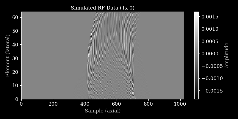
Visualize RF Data

Let’s plot the simulated RF data for the first transmit.

plot_rf(rf_data, title="Simulated RF Data (Tx 0)")

Process simulated data with zea.Pipeline

We can process the simulated RF data using a Zea pipeline to obtain a B-mode image.

pipeline = zea.Pipeline.from_default(enable_pfield=False, with_batch_dim=False, baseband=False)
parameters = pipeline.prepare_parameters(probe, scan, dynamic_range=(-50, 0))
inputs = {pipeline.key: rf_data}

outputs = pipeline(**inputs, **parameters)
image = outputs[pipeline.output_key]

image = zea.display.to_8bit(image, dynamic_range=(-50, 0))

plt.figure()
plt.imshow(
    image,
    cmap="gray",
    extent=[
        scan.xlims[0] * 1e3,
        scan.xlims[1] * 1e3,
        scan.zlims[1] * 1e3,
        scan.zlims[0] * 1e3,
    ],
)
plt.xlabel("X (mm)")
plt.ylabel("Z (mm)")
plt.title("Simulated B-mode Image")
plt.tight_layout()
plt.savefig("simulation_plot_fish.png")
plt.close()

zea: WARNING No azimuth angles provided, using zeros
zea: WARNING No transmit origins provided, using zeros
zea: DEBUG [zea.Pipeline] The following input keys are not used by the pipeline: {'center_frequency', 'xlims', 'n_el', 'zlims'}. Make sure this is intended. This warning will only be shown once.

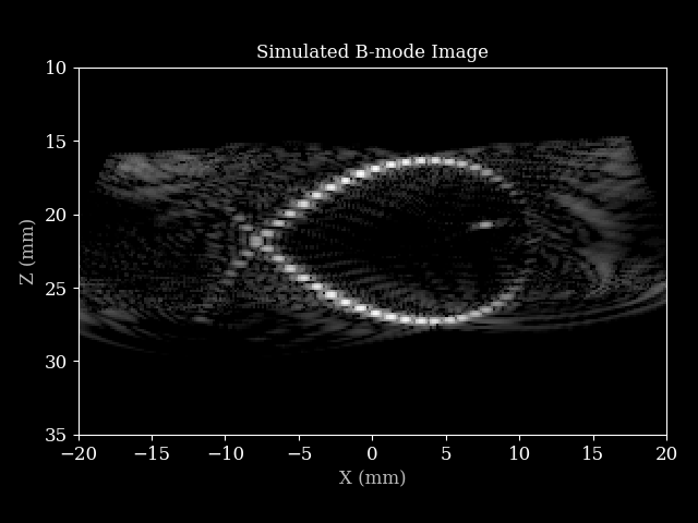
That’s it! You have now simulated ultrasound RF data and reconstructed a B-mode image using zea.

Speedup with Just-In-Time compilation (JIT)

The simulate_rf function took quite some time to compute in this example. Larger experiments with more point scatterers or acquisitions can execute very slowly. In this case, it is advised to JIT-compile the simulate_rf function. The way you do this depends on which machine learning backend (e.g., JAX, PyTorch, TensorFlow) you are using (see documentation for details). Starting with JAX, you can simply wrap the function with jax.jit as follows:

JAX

from jax import jit

simulate_rf_jit = jit(simulate_rf, static_argnames=["apply_lens_correction", "n_ax"])

Let’s execute and time the JIT versus non-JIT versions of the simulate_rf function to see the speedup.

from zea.utils import FunctionTimer

# Warm-up JIT compilation before benchmarking
simulate_rf_jit(**simulation_args)

timer = FunctionTimer()
timed_rf = timer(simulate_rf, name="simulate_rf")
timed_rf_jit = timer(simulate_rf_jit, name="simulate_rf (JIT)")

for _ in range(30):
    timed_rf_jit(**simulation_args)
    timed_rf(**simulation_args)

timer.print()

Function Timing Statistics
=====================================================================================================
Function              Mean          Median        Std Dev       Min           Max           Count
-----------------------------------------------------------------------------------------------------
simulate_rf           0.220066      0.218923      0.021850      0.189399      0.255911      30
simulate_rf (JIT)     0.004081      0.003444      0.003207      0.003159      0.020947      30

If you are using another backend, a similar approach can be taken:

PyTorch

import torch
simulate_rf_jit = torch.jit.script(simulate_rf)

TensorFlow

import tensorflow as tf
simulate_rf_jit = tf.function(simulate_rf)