Active perception for focused transmit steering

In this tutorial we will implement a basic perception-action loop to drive intelligent and adaptive focused transmit steering. We will use Diffusion Models to implement perception-as-inference, with greedy entropy minimization as our action selection policy.

For more information we would like to refer you to the paper Patient-Adaptive Focused Transmit Beamforming using Cognitive Ultrasound.

   

‼️ Important: This notebook is optimized for GPU/TPU. Code execution on a CPU may be very slow.

If you are running in Colab, please enable a hardware accelerator via:

Runtime → Change runtime type → Hardware accelerator → GPU/TPU 🚀.

%%capture
%pip install zea

import os

os.environ["KERAS_BACKEND"] = "jax"
os.environ["TF_CPP_MIN_LOG_LEVEL"] = "3"

import keras
import keras.ops as ops
import matplotlib.pyplot as plt
from matplotlib import animation
from tqdm import tqdm

from zea import init_device
from zea.models.diffusion import DiffusionModel
from zea.ops import Pipeline, ScanConvert
from zea.func import translate
from zea.data import Dataset
from zea.visualize import plot_image_grid, set_mpl_style
from zea.agent.selection import GreedyEntropy

zea: Using backend 'jax'

n_prior_samples = 4
n_unconditional_steps = 90
n_initial_conditonal_steps = 180
n_conditional_steps = 200
n_conditional_samples = 4

We will work with the GPU if available, and initialize using init_device to pick the best available device. Also, (optionally), we will set the matplotlib style for plotting.

init_device(verbose=False)
set_mpl_style()

Load dataset and model

# load generative model
model = DiffusionModel.from_preset("diffusion-echonet-dynamic")
img_shape = model.input_shape[:2]


# load camus dataset
dataset = Dataset("hf://zeahub/camus-sample/val")
data = dataset[0]["data"]["image"]
data = keras.ops.expand_dims(data, axis=-1)
data = keras.ops.image.resize(data, img_shape)
dynamic_range = (-40, 0)
data = keras.ops.clip(data, dynamic_range[0], dynamic_range[1])
data = translate(data, dynamic_range, (-1, 1))
data = data[..., 0]  # remove channel dim

zea: Searching /zea/.cache/zea/huggingface/datasets/datasets--zeahub--camus-sample/snapshots/617cf91a1267b5ffbcfafe9bebf0813c7cee8493/val for ['.hdf5', '.h5'] files...
zea: Dataset validated. Check /zea/.cache/zea/huggingface/datasets/datasets--zeahub--camus-sample/snapshots/617cf91a1267b5ffbcfafe9bebf0813c7cee8493/val/validated.flag for details.

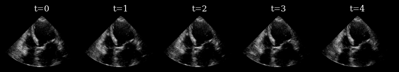
Visualize target sequence

Here we load a sequence of ultrasound frames from the CAMUS validation set. This will be our ‘ground truth’ target sequence, that the agent will need to reconstruct from a small budget of focused scan lines

scan_convert = Pipeline([ScanConvert(order=2, jit_compile=False)])
parameters = {
    "theta_range": [-0.78, 0.78],  # [-45, 45] in radians
    "rho_range": [0, 1],
}
parameters = scan_convert.prepare_parameters(**parameters)
data_sc = scan_convert(data=data, **parameters)["data"]

n_frames_to_plot = 5
fig, _ = plot_image_grid(
    data_sc[:n_frames_to_plot],
    titles=[f"t={t}" for t in range(n_frames_to_plot)],
    ncols=n_frames_to_plot,
    remove_axis=True,
    vmin=-1,
    vmax=1,
)

zea: WARNING GPU support for order > 1 is not available. Disabling jit for ScanConvert.

Simulate Focused Line Acquisition

We use a simple masking operator to simulate acquiring a set of focused lines from the tissue, where each line reveals a vertical column of pixels, in the polar domain, of the target.

def simulate_acquisition(full_frame, mask):
    measurement = full_frame[None, ...] * mask
    return measurement, mask

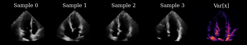
Perception-Action Loop

Initially, we have not yet acquired any measurements, so we draw samples from the prior to drive our actions.

prior_samples = model.sample(n_samples=n_prior_samples, n_steps=n_unconditional_steps, verbose=True)
scan_converted_prior_samples = scan_convert(
    data=keras.ops.squeeze(prior_samples, axis=-1), **parameters
)["data"]
posterior_variance = ops.nan_to_num(ops.var(scan_converted_prior_samples, axis=0))
fig, _ = plot_image_grid(
    list(scan_converted_prior_samples) + [translate(posterior_variance, range_to=(-1, 1))],
    titles=[f"Sample {i}" for i in range(n_prior_samples)] + ["Var[x]"],
    vmin=-1,
    vmax=1,
    cmap=["gray"] * n_prior_samples + ["inferno"],
)

90/90 ━━━━━━━━━━━━━━━━━━━━ 12s 46ms/step

Next, we implement a perception-action loop, using a greedy entropy minimization strategy to select which lines to acquire next in the sequence. Each set of generated posterior samples at time \(t\) are used as initial samples for the reverse diffusion at time \(t+1\) [1], ensuring that we generate a reconstructed sequence that is coherent over time.

[1] https://ieeexplore.ieee.org/document/10889752

frame_height, frame_width, _ = model.input_shape
action_selector = GreedyEntropy(
    n_actions=14,  # acquire 25% of measurements
    n_possible_actions=frame_width,
    img_width=frame_width,
    img_height=frame_height,
)

# select the first actions based on the prior samples
prior_samples_batched = prior_samples[None, ..., 0]  # add batch, remove channel
selected_lines, measurement_mask = action_selector.sample(prior_samples_batched)
# initialise the previous samples as the prior samples
previous_samples = prior_samples

reconstructions = []
measurements = []
for target_frame in tqdm(data):
    # perception
    measurements_t, measurement_mask_t = simulate_acquisition(target_frame, measurement_mask)
    posterior_samples = model.posterior_sample(
        measurements=measurements_t[..., None],  # add channel dim
        mask=measurement_mask_t[..., None],  # add channel dim
        initial_samples=previous_samples,
        n_samples=n_conditional_samples,
        n_steps=n_conditional_steps,
        omega=10,
        initial_step=n_initial_conditonal_steps,
    )

    # action
    selected_lines, measurement_mask = action_selector.sample(posterior_samples[..., 0])

    # gather the selected measurements and reconstructions for visualization
    reconstructions.append(posterior_samples[0])
    measurements.append(measurements_t)
    # reset the previous_samples
    previous_samples = posterior_samples

# postprocess outputs for plotting
reconstructions = ops.convert_to_tensor(reconstructions)
measurements = ops.convert_to_tensor(measurements)
selected_reconstructions = reconstructions[
    :, 0, ...
]  # choose first sample for each frame to display
reconstructions_sc = scan_convert(data=selected_reconstructions[..., 0], **parameters)["data"]
measurements_sc = scan_convert(data=measurements[:, 0, ...], **parameters)["data"]
variances_sc = scan_convert(
    data=ops.var(reconstructions, axis=1)[..., 0], **(parameters | {"fill_value": 0.0})
)["data"]
variances_sc = translate(variances_sc, range_to=(-1, 1))

Visualize the results

Finally, we visualize our reconstructed sequence, along with the selected measurements and posterior variance at each step. The agent’s goal of minizing posterior entropy is reflected in the low posterior variance throughout the sequence. You can see that the agent is quickly able to reduce the uncertainty after the first frame, when it was able to observe using acquisition of the first focused lines.

# plot image
fig, ims = plot_image_grid(
    [data_sc[0], measurements_sc[0], reconstructions_sc[0], variances_sc[0]],
    titles=["Target", "Measurements", "Reconstruction", "Variance"],
    ncols=4,
    vmin=-1,
    vmax=1,
    cmap=["gray"] * 3 + ["inferno"],
    figsize=(11, 4),
)
fig.tight_layout(pad=0)


def update(frame):
    ims[0].set_array(data_sc[frame])
    ims[1].set_array(measurements_sc[frame])
    ims[2].set_array(reconstructions_sc[frame])
    ims[3].set_array(variances_sc[frame])
    return ims


ani = animation.FuncAnimation(fig, update, frames=len(data_sc), blit=True, interval=100)
plt.close(fig)
ani.save("agent_example_reconstruction.gif")