Left ventricle segmentation

 

This notebook demonstrates how to perform left ventricle segmentation in echocardiograms using two different models within the zea framework. We apply both models on the CAMUS dataset for demonstration.

1. EchoNetDynamic

 

• Trained on the EchoNet-Dynamic dataset.

• Segments the left ventricle in echocardiograms.

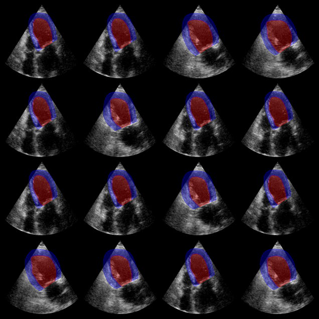
2. Augmented CAMUS Segmentation Model

 

• nnU-Net based model trained on the augmented CAMUS dataset.

• Segments both the left ventricle and myocardium (2 labels).

• State-of-the-art for left ventricle segmentation on CAMUS.

‼️ Important: This notebook is optimized for GPU/TPU. Code execution on a CPU may be very slow.

If you are running in Colab, please enable a hardware accelerator via:

Runtime → Change runtime type → Hardware accelerator → GPU/TPU 🚀.

%%capture
%pip install zea
%pip install onnxruntime # needed for the Augmented CAMUS Segmentation Model

import os

os.environ["KERAS_BACKEND"] = "tensorflow"
os.environ["TF_CPP_MIN_LOG_LEVEL"] = "3"

from zea import init_device
import matplotlib.pyplot as plt
from keras import ops
from zea.backend.tensorflow.dataloader import make_dataloader
from zea.visualize import plot_shape_from_mask
from zea.func import translate
from zea.visualize import plot_image_grid, set_mpl_style

init_device(verbose=False)
set_mpl_style()

zea: Using backend 'tensorflow'

Load CAMUS Validation Data

We load a batch of images from the CAMUS validation set. This batch will be used as input for both segmentation models.

n_imgs = 16
INFERENCE_SIZE = 256  # Used for both models
val_dataset = make_dataloader(
    "hf://zeahub/camus-sample/val",
    key="data/image_sc",
    batch_size=n_imgs,
    shuffle=True,
    image_range=[-45, 0],
    clip_image_range=True,
    normalization_range=[-1, 1],
    image_size=(INFERENCE_SIZE, INFERENCE_SIZE),
    resize_type="resize",
    seed=42,
)

batch = next(iter(val_dataset))
rgb_batch = ops.concatenate([batch, batch, batch], axis=-1)  # For EchoNetDynamic

zea: Using pregenerated dataset info file: /root/.cache/zea/huggingface/datasets/datasets--zeahub--camus-sample/snapshots/617cf91a1267b5ffbcfafe9bebf0813c7cee8493/val/dataset_info.yaml ...
zea: ...for reading file paths in /root/.cache/zea/huggingface/datasets/datasets--zeahub--camus-sample/snapshots/617cf91a1267b5ffbcfafe9bebf0813c7cee8493/val
zea: Dataset was validated on September 29, 2025
zea: Remove /root/.cache/zea/huggingface/datasets/datasets--zeahub--camus-sample/snapshots/617cf91a1267b5ffbcfafe9bebf0813c7cee8493/val/validated.flag if you want to redo validation.
zea: WARNING H5Generator: Not all files have the same shape. This can lead to issues when resizing images later....
zea: H5Generator: Shuffled data.
zea: H5Generator: Shuffled data.

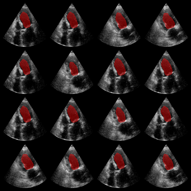
Inference with EchoNetDynamic Model

We first run inference using the EchoNetDynamic model, which expects RGB input images. The model was trained on the EchoNet-Dynamic dataset, but here we apply it to CAMUS data for demonstration.

from zea.models.echonet import EchoNetDynamic

# Load model
model_echonet = EchoNetDynamic.from_preset("echonet-dynamic")

# Inference (expects RGB input)
masks_echonet = model_echonet(rgb_batch)
masks_echonet = ops.squeeze(masks_echonet, axis=-1)
masks_echonet = ops.convert_to_numpy(masks_echonet)

# Visualization
batch_vis = translate(rgb_batch, [-1, 1], [0, 1])
fig, _ = plot_image_grid(batch_vis, vmin=0, vmax=1)
axes = fig.axes[:n_imgs]
for ax, mask in zip(axes, masks_echonet):
    plot_shape_from_mask(ax, mask, color="red", alpha=0.4)

plt.savefig("echonet_output.png", bbox_inches="tight", dpi=100)
plt.close(fig)

EchoNetDynamic segmentation results:

The red overlay shows the predicted left ventricle mask for each image.

Inference with Augmented CAMUS Model

Now we use the Augmented CAMUS nnU-Net model, which segments both the left ventricle and myocardium (2 labels). The model expects input in NCHW format (batch, channels, height, width).

from zea.models.lv_segmentation import AugmentedCamusSeg
import numpy as np

# Load model and weights
model_camus = AugmentedCamusSeg.from_preset("augmented_camus_seg")

# Prepare input for ONNX (NCHW: batch, channels, height, width)
batch_np = ops.convert_to_numpy(batch)
onnx_input = np.transpose(batch_np, (0, 3, 1, 2))

# Inference
outputs_camus = model_camus.call(onnx_input)
outputs_camus = np.array(outputs_camus)
# Predicted class = class with the highest score for each pixel
masks_camus = np.argmax(outputs_camus, axis=1)  # shape: (batch, H, W)

# Visualization: show both LV (label 1) and myocardium (label 2)
fig, _ = plot_image_grid(batch_np, vmin=-1, vmax=1)
axes = fig.axes[:n_imgs]
for ax, mask in zip(axes, masks_camus):
    # LV: label 1, Myocardium: label 2
    plot_shape_from_mask(ax, mask == 1, color="red", alpha=0.3)
    plot_shape_from_mask(ax, mask == 2, color="blue", alpha=0.3)

plt.savefig("augmented_camus_seg_output.png", bbox_inches="tight", dpi=100)
plt.close(fig)

Augmented CAMUS segmentation results:

Red: left ventricle mask. Blue: myocardium mask.